In this tutorial, we will learn how to solve the weighted MaxCut problem which is a combinatorial graph theory problem.

The MaxCut problem is an optimization problem in which the nodes of a given undirected graph have to be divided in two sets such that the number and weight of edges connecting a color node with another color node are maximized (the color is what distinguishes one set of nodes from the other) In the following diagram we will be using green and blue nodes. Read this article to find out more about the exact details of the problem.

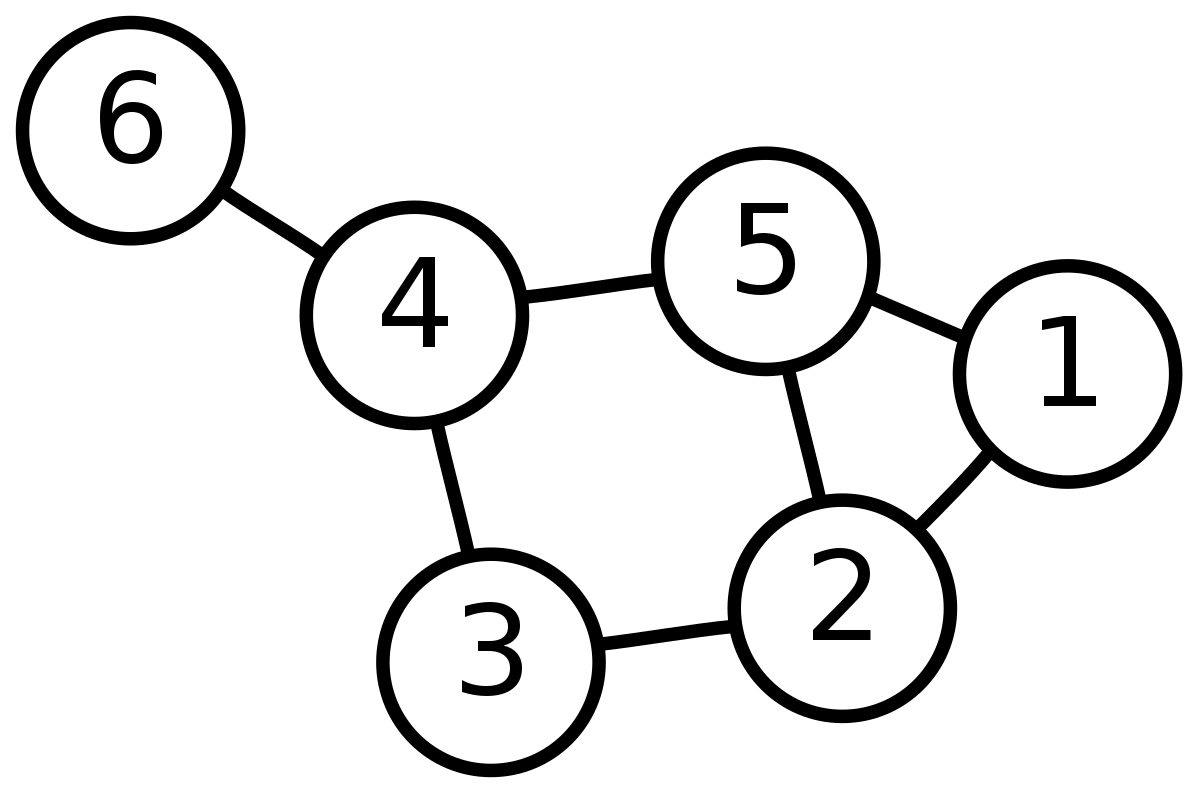
Each graph consists of a set of edges and nodes. In the following image, the nodes are 1,2...6 and the edges are the lines joining the nodes

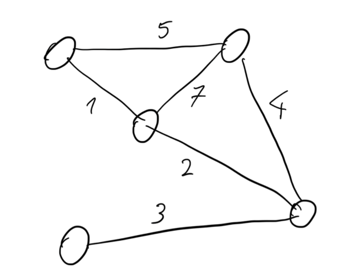
Given a graph with weights, which are essentially values assigned to each edge of the graph, the maxcut problem should output the following solution.

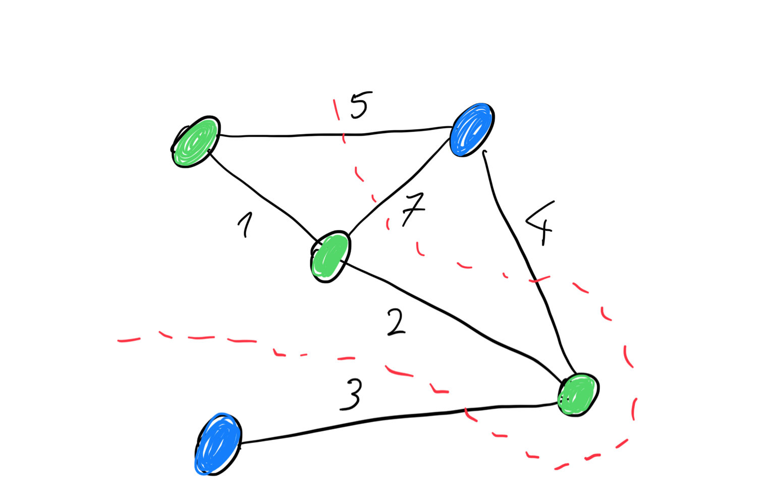
Where we will find a path or a cut separating the green and the blue nodes such that the edges going between the two sets have the biggest possible weight. The MaxCut problem can be solved using the Quantum Approximate Optimization Algorithm, which is what we will be exploring.

import pennylane as qml
from pennylane import numpy as np

Step One : Initialize a graph in PennyLane

n_wires is a parameter which denotes number of nodes in the graph. This will be equal to the number of qubits we will be using in our circuit. We will also declare edges set which consists of the edges in the graph and the corresponding weights attached to each edge.

n_wires = 3
graph = [(0,1), (1,2), (0,2)]
weight = [10, 1, 10]

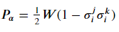
Our goal is to separate the whole set of nodes in two subsets X and Y such that the sum of weights of edges traversing between them have the maximum possible value. Or, we have to find a partition through the whole graph, such that sum of weights of edges that the partition passes becomes the maximum among all possible partitions.

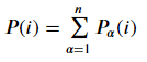
The equation above specifies a particular partition of the graph where

represents the weight at each node i(if the partition passes through the node, 0 otherwise), where it is a piecewise function and the summation operator represents the sum of all the weighted edges.

Step Two : Define the unitary operators

We will define the partition in terms of computational basis states and operators acting on the states where the a th edge is the edge connecting jth and k nodes and will be equal to P of a if partition goes between jth and kth nodes and equal to 0 if doesn't pass.

We are converting the circuit into a superposition state by applying the hadamard gate on each qubit.

The circuit defined above can be represented as consisting of L layers where

are two gates on each layer associated with two different parameters a and b. The whole circuit will thus have 2L parameters. We will define it as a Rx gate as it is implemented on two nodes connected by an edge in the graph. U2 will consist of RZ gate in between two CNOT gates.

def U_1(param1):
    for qubit in range(n_wires):
        qml.RX(2*param1, wires=qubit)

def U_2(param2):
    for i in range(n_wires):

        qubit1 = graph[i][0]
        qubit2 = graph[i][1]
        w = weight[i]
        
        qml.CNOT(wires = [qubit1, qubit2])
        qml.RZ((-1)*w*param2, wires = qubit2)
        qml.CNOT(wires = [qubit1, qubit2])

Step Three : Perform Computational Basis Measurement

To measure the values of the qubits we will apply the hermitian operator where the eigenvalues of the operator are the values of the measured qubits.

def computational_basis_measurement(wires):
    n_wires = len(wires)
    return qml.Hermitian(np.diag(range(2 ** n_wires)), wires=wires)

Step Four : Create and compile the circuit

Create a device on which to execute the circuit where the number of wires is same as number of nodes present in the graph or n_wires as we defined above.

dev = qml.device("default.qubit", wires=n_wires, analytic=True, shots=1)

To measure the expectation value, we will define a Pauli Z operator and take the kronecker product.

pauliZ = [[1, 0], [0, -1]]

pauliZ_kron = np.kron(pauliZ, pauliZ)

For compiling the entire circuit we will apply the functions and operators.

Initially, the state of each qubit is initialized to |0> by default. We will need to apply a Hadamard gate to create superposition and call the U1 and U2 gates. Then we will measure the expectation value of the edges using the kronecker product of the Pauli Z gate using the expval function.

@qml.qnode(dev)
def circuit(param1, param2, edge=None, layers=1):

    for qubit in range(n_wires):
        qml.Hadamard(wires = qubit)

    for l in range(layers):
        U_1(param1[l])
        U_2(param2[l])

    if edge is None:
        return qml.sample(computational_basis_measurement(range(n_wires)))

    return qml.expval(qml.Hermitian(pauliZ_kron, wires=edge))

Step Five : Optimization of the Circuit

We will optimize the circuit we just created by calling the AdagradOptimizer with step size 0.5. This optimizer uses the Adagrad algorithm which is a variant of gradient descent. We will then return lists of bitstrings that were measured after executing the circuit over multiple trials, check this for more information on why this technique works.

def optimizemaxcut(layers = 1):

    dev = qml.device("default.qubit", wires=n_wires, analytic=True, shots=1)

    @qml.qnode(dev)
    def circuit(param1, param2, edge=None, layers=1):

        for qubit in range(n_wires):
            qml.Hadamard(wires = qubit)

        for l in range(layers):
            U_1(param1[l])
            U_2(param2[l])

        if edge is None:
            return qml.sample(computational_basis_measurement(range(n_wires)))

        return qml.expval(qml.Hermitian(pauliZ_, wires=edge))


    init_params = 0.01 * np.random.rand(2, layers)



    def objective_func(params):

        param1 = params[0]
        param2 = params[1]

        score = 0
        
        for i in range(n_wires):
            score -= 0.5 * (1 - weight[i] * circuit(param1, param2, edge=graph[i], layers=layers))

        return score

    optimizer = qml.AdagradOptimizer(stepsize = 0.5)

    params = init_params

    n_iters = 120

    for iter in range(n_iters):
        params = optimizer.step(objective_func, params)

    n_samples = 100
    bit_strings = []

    for i in range(n_samples):
        param1 = params[0]
        param2 = params[1]
        bit_string = int(circuit(param1, param2, 
                                 edge = None, 
                                 layers = layers))
        bit_strings.append(bit_string)


    return ((-1)*objective_func(params), bit_strings)

Step Six : Executing the circuit

We will execute the circuit layer by layer. Since we have 3 nodes, we will create 6 layers.

n_wires = 3
graph = [(0,1), (1,2), (0,2)]
weight = [10.0, 1.0, 10.0]
result_layer_1 = optimizemaxcut(layers = 1)
result_layer_2 = optimizemaxcut(layers = 2)
result_layer_3 = optimizemaxcut(layers = 3)
result_layer_4 = optimizemaxcut(layers = 4)
result_layer_5 = optimizemaxcut(layers = 5)
result_layer_6 = optimizemaxcut(layers = 6)

Solution: The partitioned graph

We can try out different graphs for instance

n_wires = 5
graph = [(0,1), (0,2), (1,2), (1,3), (2,3), (3,4)]
weight = [5.0, 1.0, 7.0, 4.0, 2.0, 3.0]

This 5 qubit graph will get a partition.

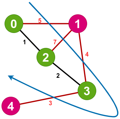
Where we can verify that the partition between the different colored nodes is maximum as the sum of the edges that pass through the cut is the maximum.